Capturing the flash spectrum during a solar eclipse offers invaluable insights into the Sun’s outer layers like the chromosphere and the mesosphere. To harness this data, it is essential to extract and process specific video frames effectively. This blog post will guide you through the steps of extracting a frame from a video, isolating the solar spectrum, and visualizing the obtained spectral lines with few lines of Python code.
Step 1: Extract a Frame from the Video
We’ll use OpenCV for this purpose
        import cv2 # OpenCV
        import matplotlib.pyplot as plt
First, we need to capture a frame from the video where the flash spectrum of the solar eclipse is clearly visible.
        # Path to the video file
        video_path = r"FlashSpectrumVideo.MOV"

        # Read the frame
        cap = cv2.VideoCapture(video_path)
        success, img = cap.read()

        if success:
            print("Frame captured successfully")
        else:
            print("Failed to capture frame")


        # Display the captured frame for verification
        cv2.imshow("Captured Frame", img)
        cv2.waitKey(0)
        cv2.destroyAllWindows()

Note that the frame has ben taken at the moment close to C2 and the spectrum is the one of the outer layer of the Sun disappearing behind the last valley of the Moon limb.
The Sun and the spectrum in our video are not centered, so we can crop it a bit for aesthetic reasons.
        # Crop the frame vertically and convert it to grayscale
        img = img[0:1500, 0:img.shape[1]]  # Adjust crop as necessary

        # Print the shape of the cropped image
        print("Cropped image shape:", img.shape)
After running this segment of code, you should see an output similar to this in your console.
Cropped image shape: (1500, 3840, 3)
This output provides the dimensions of the cropped frame (height, width, and the number of color channels).
Moreover it is necessary to convert it to grayscale in order to get the intensity of the light in every pixel (*see also note1).
gray = cv2.cvtColor(img, cv2.COLOR_BGR2GRAY)
Step 2: Sample the Frame to Extract the Spectrum
Next, we’ll sample the grayscale frame along a horizontal line to isolate the spectrum, visualizing it with the matplotlib library.
In our image the spectrum of the Bailys bead is at the vertical position 802.
Moreover we want to consider that the spectrum doesn’t cover the whole width of the image, but say from pixel 2000 to 4000
        # Specify the horizontal line's vertical position
        y1 = 802  # Adjust this value based on your frame content

        # Sample the frame along the specified line
        L = gray[y1, :]

        # Draw a green line on the original frame for reference
        cv2.line(img, (2000, y1), (4000, y1), (255, 255, 0), 1)

        # Plot the intensity of the sampled line to visualize the spectrum
        fig, ax = plt.subplots(figsize=(8, 4))
        plt.plot(L)
        plt.title("Solar Spectrum")
        plt.xlabel('Pixel Position')
        plt.ylabel('Intensity (Normalized)')
        plt.xlim([2000, 4000])  # Adjust xlim based on your spectrum region
        plt.show()
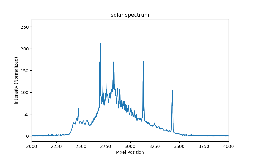
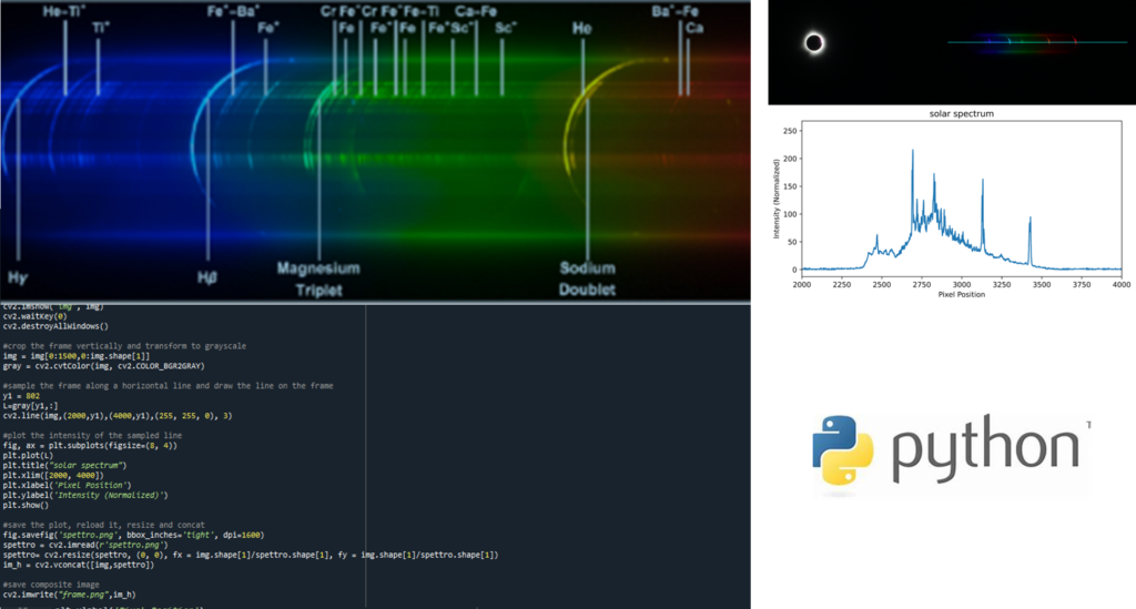
In the chart it is possible to see the spectrum of the Sun. The peaks of Hα, Hβ, He, the Sodium doublet the Magnesium triplet are clearly visible. With them it is also possible to change the X-axis scale from pixel to wavelength
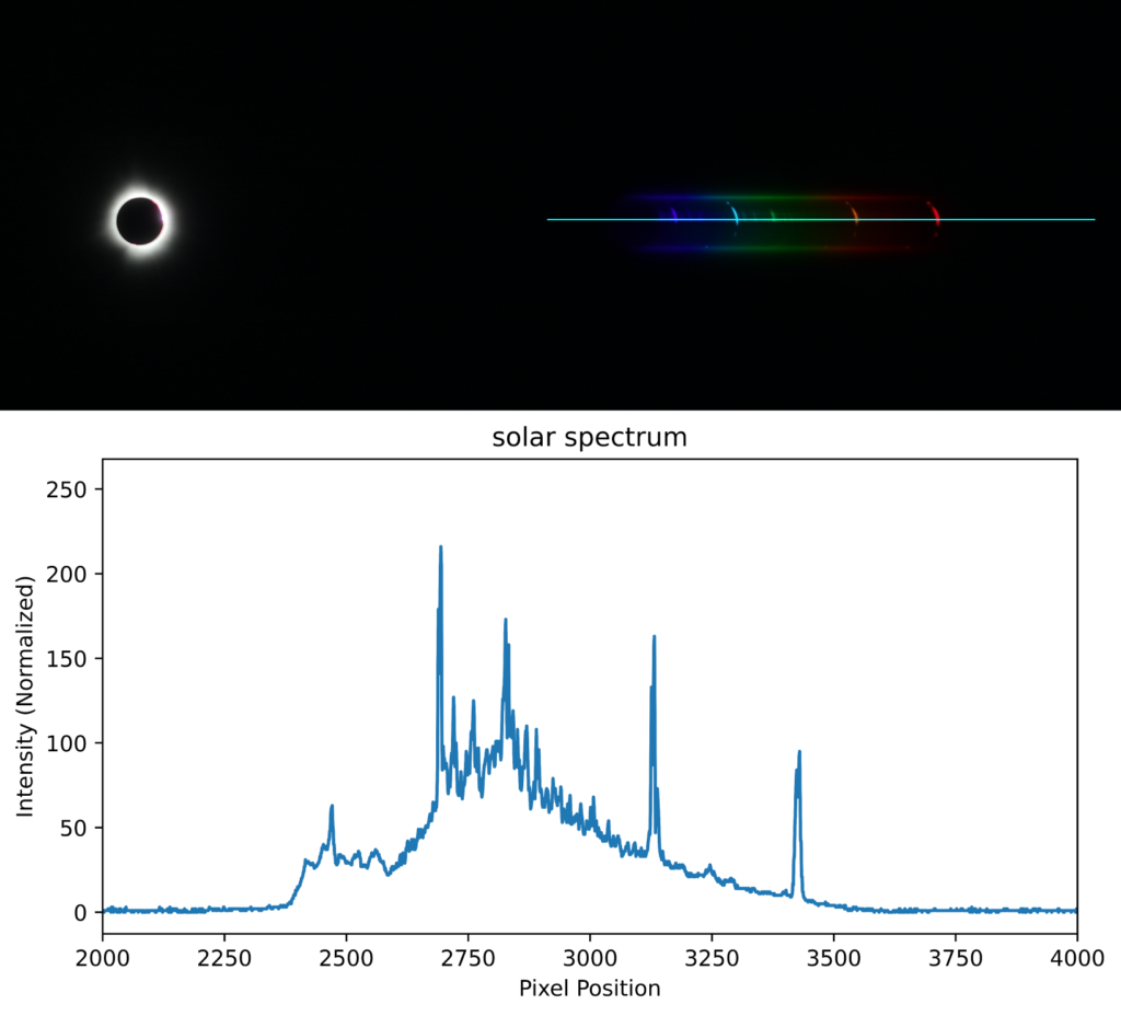
Step 3: Save and Combine the Results
We save the plotted spectrum, resize it, and concatenate it with the original image for a comprehensive view.
        # Save the spectrum plot
        fig.savefig('spectrum.png', bbox_inches='tight', dpi=1600)

        # Reload the saved plot and resize it to match the original image's width
        spectrum_img = cv2.imread('spectrum.png')
        spectrum_img = cv2.resize(spectrum_img, (img.shape[1], int(spectrum_img.shape[0] * (img.shape[1] / spectrum_img.shape[1]))))

        # Concatenate the original image with the spectrum plot vertically
        composite_img = cv2.vconcat([img, spectrum_img])

        # Save the final composite image
        cv2.imwrite("composite_spectrum_frame.png", composite_img)
        print("Composite image saved as 'composite_spectrum_frame.png'")
Conclusion
In this post, we’ve walked through the essential steps to capture a frame from a solar eclipse video, extract and visualize the solar spectrum, and consolidate the results into a single image. This process enables a detailed examination of the Sun’s outer layers spectrum, revealing valuable data about its composition and behavior.
By leveraging readily available Python libraries such as OpenCV and Matplotlib, the integration of video data analysis becomes accessible to everybody. In future post we will go across additional analysis like specific wavelength region sampling, light curve extraction, what to do in case the spectrum is not horizontal,
Note1: in this post we converted an RGB image into greyscale to get the intensity. It is not completely correct if the original image has a been gamma corrected. In this case it is necessary to remove the correction to get the luminance of the image proportional to the light intensity that hit the sensor